What after Gradient Descent

This blog covers some algorithms of Deep Learning such as Gradient Descent and their limitations. It’s broadly divided into two sections. The first one discusses different ways to calculate the gradient descent or any such algorithm and the later section discusses about the limitations of the algorithms and what can be used next. In the end you’ll get to know the deadliest combination that every deep learning specialist should know.

Calculating Gradient Descent:

Gradient Descent can be calculated using below mentioned three ways:

  1. Batch
  2. Mini Batch
  3. Stochastic

Loss Function:

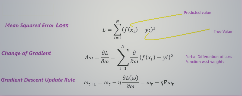
In Batch Gradient Descent, the parameters(weights) are updated after a pass over the entire data (one epoch). So, in case of very large number of records, updates happen less, and large number of epochs are required to achieve minimal loss.

In Stochastic Gradient Descent, the parameters are updated after pass over single data point. It leads to large number of parameter updates in a single run over the entire data (one epoch). This eventually causes a lot of oscillations in the loss, as each data point directs the gradient as per its understanding without considering other points.  Also, Stochastic gradient descent is not true but an approximate of the gradient value as the true value can be derived only considering the whole data.

In Mini Batch Gradient Descent, the parameters are updated after one pass over the mini batch (usually a power of 2).  This reduces the number of oscillations and also serves to update the parameters more often than the Batch Gradient Descent. The size of mini batch is usually 32,64,128.

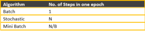
Here N = No. of data points, B = size of Mini Batch

Utilising Gradient Descent:

Gradient Descent can be used using below mentioned algorithms:

  1. Momentum Based Gradient Descent
  2. Nesterov Accelerated Gradient Descent
  3. Adagrad
  4. RMSProp
  5. Adam
So, if we substitute $ \frac{\partial y}{\partial x} $ in the gradient descent algorithm, we observe that the rate of decrease of weights(optimization) is higher in case of steep slopes, while the same is very less in case of gentle slope.

So, in scenario where gentle slope is encountered the gradient is very small and algorithm learns very slowly, consuming large number of epochs.

This limitation of Gradient Descent can be overcome by the implementation of Momentum Based Gradient Descent.


Momentum Based Gradient Descent (MBGD):

In Momentum Based Gradient Descent, the history component is taken into consideration to compute the gradient:

Since the value of γ lies between 0 & 1. Higher the power of γ, lower the value of its term. This is called as Exponentially Decaying Average.

So, the value of current gradient is higher than the previous one.

Advantages: Even in regions having gentle slopes, momentum based Gradient Descent is able to take larger steps because of its momentum.

Disadvantage: Due to higher momentum, the algorithm runs past the minima and takes a lot of u turns to achieve there. It overshoots the target due to momentum, showing lots of oscillation.

But still converges faster than the plain Gradient Descent.

To overcome the limitation of Momentum Based Gradient Descent, Nesterov Accelerated Gradient Descent can be implemented.

Nesterov Accelerated Gradient Descent (NAG)

The disadvantage of Momentum Based gradient Descent was because the present gradient is used to determine the future movements (one step ahead). In any scenario, it needs to move double the distance, for history(momentum) and current gradient

To overcome this shortcoming, NAG first moves as per the history component, calculates the gradient at the temporary point and then moves forward or backward on the present gradient. This reduces the overshooting and hence the oscillations.

Advantages: Looking ahead helps NAG in correcting its course quicker than MBG. Hence oscillations are smaller and chances for escaping the minima is also smaller.


In case of data with many features, Plain Gradient Descent, Momentum Based Gradient Descent and Nesterov Accelerated Gradient Descent fail to reach the global minima. This is because of the similar learning rate for all the features be it either dense or sparse.

Now what is a Dense Features: are the ones which receive a lot of updates in an epoch while Sparse features receive very a smaller number of updates (smaller number of records exhibiting the feature)

So, the algorithm would need to update the learning rate differently for dense and sparse features.

Adagrad:

It decays the learning rate of parameters in proportion to their update history (fewer updates, lesser decay). Just as we needed to handle learning rate for Dense and Sparse features.

The denominator term  is high for features which receives a lot of updates in the past (dense features) while smaller number of updates for sparse features.


Advantages: Parameters corresponding to Sparse features get better updates

Disadvantages: The learning rate decays very aggressively as the denominator grows (not good for parameters corresponding to dense features). Adagrad is unable to reach the minimal loss point due to rapid decay of learning rate.

RMSProp

Prevents the denominator (vt) to grow aggressively for dense features. For sparse features, the value of history will still be considered.

RMS Prop overcomes the problem of Adagrad by being less aggressive on decays.

Adam:

Combines the idea in Momentum Based Gradient Descent and RMSProp.

Momentum Based Gradient Descent – uses history to compute current update

RMSProp – history is being used to change the learning rate.


Now, the Most popular combination of all the algorithms discussed above –

Adam with Mini Batch


Happy Reading!!!

You may also like...

Leave a Reply

Your email address will not be published. Required fields are marked *